 In his keynote at the Lean Kanban Central Europe 2012 conference David J. Anderson proposed a new metric for Kanban Systems, which is supposed to provide an answer to the big organizational governance question: “How do you choose where to place a piece of work or project?” The idea is to measure the pull transactions per volume (persons or units of currency) in a Kanban System, which shall tell us how liquid it actually is. There is an analogy to the liquidity of the markets from the investment banking domain: the more liquid a market is the higher the trust is. According to David:
> …Measuring and reporting system liquidity is important to building trust to enable a probabilistic approach to management of knowledge work and hence elimination of wasteful economic overheads facilitating the comfort mechanisms inherent in the existing pseudo-deterministic approach to management. System liquidity provides an important indicator, solving the governance challenge of selecting the best vendor or department to process a work order…
In his keynote at the Lean Kanban Central Europe 2012 conference David J. Anderson proposed a new metric for Kanban Systems, which is supposed to provide an answer to the big organizational governance question: “How do you choose where to place a piece of work or project?” The idea is to measure the pull transactions per volume (persons or units of currency) in a Kanban System, which shall tell us how liquid it actually is. There is an analogy to the liquidity of the markets from the investment banking domain: the more liquid a market is the higher the trust is. According to David:
> …Measuring and reporting system liquidity is important to building trust to enable a probabilistic approach to management of knowledge work and hence elimination of wasteful economic overheads facilitating the comfort mechanisms inherent in the existing pseudo-deterministic approach to management. System liquidity provides an important indicator, solving the governance challenge of selecting the best vendor or department to process a work order…
In layman’s terms, the probability of getting desired outcome is higher if I work with the team with the highest liquidity.
Liquidity for Kanban Systems
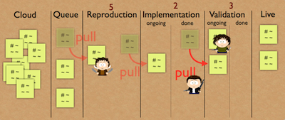
Imagine the Kanban System as a market where the transactions are the pulls. In this context the liquidity of a Kanban System is the number of pull transactions in a given time period (which is three in the example above). There is a normalized form in which the number of pull transactions is divided by the number of team members (or currency) in a given time period. I’m going to use the normalized form in the rest of this post, but will leave out the word “normalized” when referring to it for simplicity.

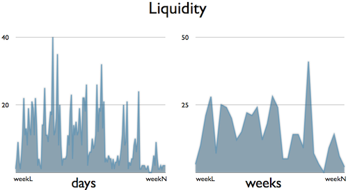
At the end of his talk, David challenged the Kanban community to measure the liquidity in their organizations and collect as much information as possible to see how the idea works in practice. I was curious about it, so I took the data from my “Measure and Manage Flow in Practice” talk ([1]) and calculated the liquidity of an old team of mine ([2]). I use the word “calculated” and not “measured” on purpose: my results weren’t entirely measured so they’re not solid enough. Back then I was collecting data for a different purpose and therefore I was missing some details which I had to figure out by using calculations, and this is not the way to do accurate measurements. Additionally, I didn’t remember the entire context, which made it hard to explain the data. Nevertheless, I think the result of my calculations is good enough to start with, so here is it:
The matching CFD chart:
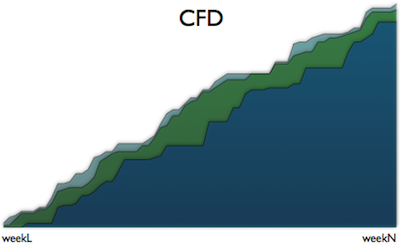
Towards the end the CFD shows some stability, however the liquidity is still moves up and down. I don’t have a good explanation, so I’d rather wait for the real measurements to provide more details about this phenomenon.
Unclear relationship between liquidity, lead time and throughput
At the moment I dare to state that the connection between liquidity, lead time and throughput is not clear yet. I cannot say that a team with higher liquidity will deliver faster or deliver more. For example, there was another team where we had a separate column for code review. After long discussions we decided to merge the code review and development columns and made the code review a part of the definition of done. I clearly remember that the lead time and the throughput did not change, however if I had calculated the liquidity I would have ended up with a lower number, because fewer columns on the board means fewer pull transactions.
This statement isn’t one hundred percent accurate either, because pull transactions won’t necessarily happen linearly, by pull after pull. Pull transactions can happen in parallel, completely unrelated to each other. Imagine that you have to do a work item and you have five columns on your board. This means that your liquidity will be five if you work only on that work item and finish it within the given time period (the number of pull transactions to get a task done is equal to the number of columns you have on your board). If you take away a column, your liquidity will be four if you follow this linear thinking. However, with fewer columns you can reduce the inventories and waiting times, so you may find some time to pull another item somewhere else on the board, so you might have a liquidity of five again. This works the other way around as well: if you need an extra column (like when we had to create verification and validation columns instead of a single testing column) you may increase your liquidity, but you may need more time to pull work items forward, so time-wise you won’t gain that extra in your liquidity.
Concerning throughput, have a look at the following charts:
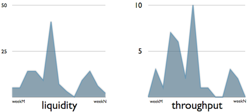
They are quite the same, but not really. There is a noticeable gap in throughput although there were multiple pulls at the very same time. Since my data comes from calculations I don’t know too much about the context, but an infinite queue on the board can explain the difference (an infinite queue is a specific column which has no WIP limit and works as an unlimited inventory): the team pushed work items into that queue more frequently than they pulled form it. In this case the liquidity will be high because of the frequent pushes, but the throughput will be low because of the rare pulls.
What liquidity is telling me at the moment
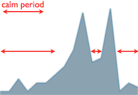
At the moment I see liquidity as an energy level indicator. In order to keep this level relatively high, the team needs to continuously improve itself (this is the fuel which is necessary to create energy). When liquidity drops or increases we know something is happening. For example, you can spot a recurring pattern (the chart on the left) in the first daily chart. There is a calmer period, which is followed by a spike and then a drop. A little bit later, there is an almost equally large spike and a calm period again. First I thought that this phenomenon happened around the dates when we had deliveries, but as far as I remember we rarely worked that much before deliveries (high number of pull transactions may indicate high workload, too). However, we had an infinite queue after implementation - I remember that clearly -, which we emptied (first spike) when we were physically unable to put more work items into it. After that we put the implemented work items into the empty queue and pulled them forward (second spike) so that we could continue the implementation (the longer calm periods) with a clean sheet.
Calculation and measurement issues
I’ve already written about the problems that infinite queues in the middle of the flow can cause, but there are more gotchas, which may make the measurements hard to perform.
The first issue is with the expand and collapse method: a couple of times, we broke down a large work item into smaller pieces and worked only with those, but at the validation phase we merged them back together. My common sense would dictate to use the pull transactions of the broken down work items, but the breakdown process is really team-specific, which may make the comparison of teams (this is the purpose of the liquidity measurements) less possible or accurate. On the other hand, if a team can break down work items in an efficient way, then that team may be better than other teams.
The second issue appears when the team rejects work items and moves them back on the board. In this case the number of pull transactions on those work items can be easily doubled if they moved back to the beginning of the board.
The last issue has nothing to do with measurements (or calculations) directly, but may cause some trouble later: the changing number of the columns and the people in the team. I’ve already written about the issues with the number of columns, and my pessimistic half has already visualized teams arguing about having more columns just to have the chance of achieving a higher liquidity instead of improving their ways of working. Additionally, the number of columns and the number of team members were changing frequently in the observed time period (for example in my case I calculated about five column changes and six changes in the number of persons in the team), and I don’t know how this change will affect the liquidity-based comparisons in the future.
Liquidity by work item size
Finally, I was curious how the liquidity by work item size chart looked like:
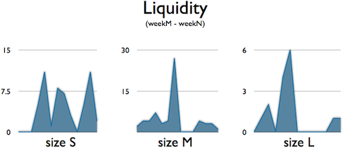
It seems that the smaller the items are, the more pull transactions are in the system, but this needs to be investigated further. I’ve already written about expand and collapse and I’m wondering if there are any connections here. In theory there is one, but I’d rather wait for some evidence from measurements before jumping to any conclusions.
The first comparison
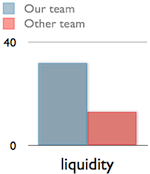
I managed to find a picture of another team, calculated their liquidity and compared it to ours (check out the chart on the right, which covers two weeks). As you can see, their liquidity was way lower than ours, but they were more trusted inside the whole organization. This might be important in the future: the measured data or scientific proof such as liquidity won’t change cognitive biases automatically. I’m certain that no matter what our team would have done, the other team had been in favor. Nevertheless, I see a great potential in liquidity for Kanban Systems, because besides the potential in comparison, liquidity provides more details about the internal affairs of a team.
Update: you can find David’s own post about liquidity on his blog.
Notes
-
I used the data behind the CFD (Cumulative Flow Diagram) and some pictures from the material of the talk
-
The pictures provided the number of columns of our boards at the time when they had been taken. I used this information to calculate the number of pull transactions, because the number of pull transactions of a finished work item was equal to the number of columns when the work item had been done. I used the lead time (done - started) to figure out when the pull transactions had happened: I evenly distributed the number of pull transactions along the working period
comments powered by Disqus