In my throughput post I was writing about a piled up inventory of work items which is created when the throughput (output) is lower than the demand (input). These work items are visible, they are on the Kanban board, and we call them aging work items. I’m not sure where the name comes from but I think it relates to the fact that these work items are staying longer in the flow (manufacturing of software process) than some others, they are usually stationary, and therefore they start aging. The aging work items are quite dangerous in terms of software development and also in terms of manufacturing.
First, they make it really hard to know the real output of a team. If you remember the example from the throughput post after a while the team had so many aging items that they couldn’t take new work items. Of course, you can throw away aging work items, but these were important once and the team invested time and effort into bringing them to where they are now. Check out the chart on the right. It shows the demand, the throughput, and the actual number of aging items. Without considering aging items we can assume that last week the team’s throughput was 7 work items, which is true, but they could only finish 5 new work items. If the team decides to take more work items in this condition, their throughput of new work items won’t change. Every week they will have at least as many aging work items as the week before, their actual speed regarding new work is 5 work items per week, so a growth in demand will only increase the number of aging items. They simply cannot work faster because of them. The solution is counterintuitive. They have to decrease the demand in order to increase throughput. In other words they need to finish the aging work items, or at least lower their number. This will lower their throughput but this throughput won’t have an invisible component.
Second, if you use velocity or throughput for forecasting, the aging items can make it inaccurate. If you know that you can deliver ‘N’ items in ‘M’ days/weeks/months you can assume that the lead time of an item is shorter or equal to ‘M’. For example, if you deliver 10 features a month you can assume that you need maximum one month to deliver one feature. If you know about aging work items you know that this assumption may be wrong. If you have at least one aging item among the delivered features, you have one item whose lead time is actually longer than ‘M’. If you draw a distribution chart of lead times (on the right) you can see that there the majority of lead times are shorter than or equal to ‘M’, however there are actually several examples of longer lead times. In the basic forecasting post I mentioned why it is more safe to use the 85%-100% range of the lead time distribution (it is more likely that you’ll deliver before the longest lead time than at the average or median lead time), and if you work under the assumption above (lead time <= ‘M’) you may fail your commitment. So, if it is possible don’t use velocity or throughput for forecasting, use lead time distribution.
Let’s see a real example. This is a throughput diagram of the team:

And the board:
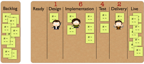
It seems that the team is improving: it outputs more and more work items. However they are in trouble now. Their current throughput is 7 work items a week, but they have 9 work items on their Kanban board. This means that they cannot take more work for at least two weeks until they get rid of all the aging items. The problem is that the team has a deadline in three weeks and their backlog has more than 10 cards.
Aging items aren’t unique, we all have them and will have in the future. The key is to find them and solve them one by one. An easy way to find them is to check how long the work items have been staying on the Kanban board. You are looking for those items that have been longer on the Kanban board than the length of the release cycle. Look for them at least once a week and talk to your team to figure out what to do with them.
comments powered by Disqus